Analyze your
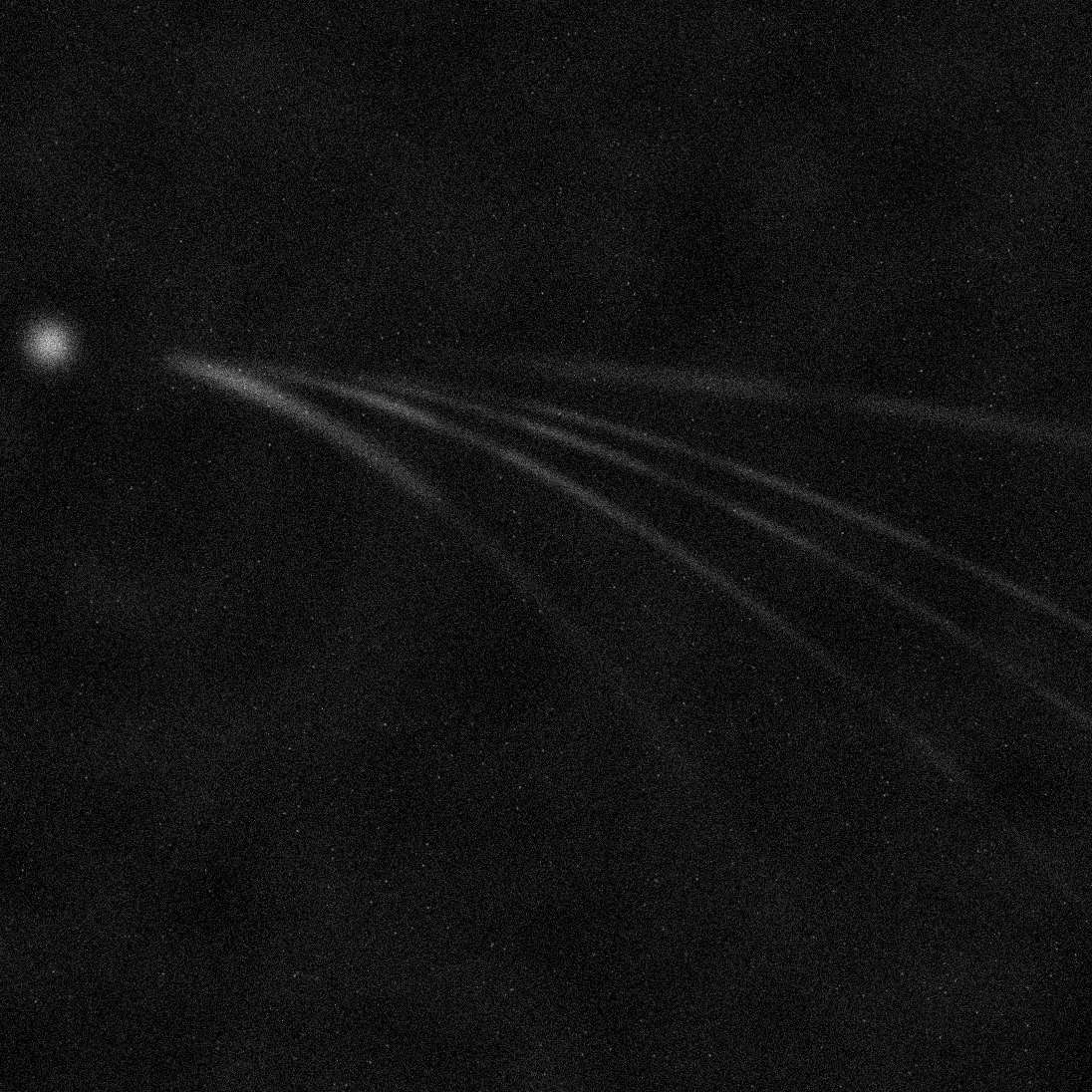
Thomson spectrometer image
Upload a raw detector image—the pipeline rotates and flips it automatically into the analysis frame—and leave the fitting, processing and plots preparation to us.
Drop image here
PNG, JPEG, TIFF or BMP — or click to browse
How the pipeline works
Oblisk turns a single Thomson parabola detector image into labelled ion tracks and energy spectra. Electric and magnetic fields in the spectrometer separate ions by charge-to-mass ratio; each species draws a distinct parabola on the plate. The software crops and denoises the image, finds smooth streaks, aligns the detector frame, fits curvature, assigns species, then integrates flux along each parabola to build dN/dE histograms.
- Preprocess — ROI crop (neural detector), then U-Net or morphological denoising.
- Background — Estimate a uniform background and subtract it for sampling.
- Traces — Enhance streaks, track line centers, smooth polyline outliers.
- Alignment — Fit origin, rotation, and axes so tracks match canonical parabolas.
- Classify — Compare fitted curvature to species ladders from your spectrometer model.
- Spectra — Sample intensity along theoretical tracks and map position to ion energy.
Interactive detector preview
Same viewer as on the results page — hover a track for species and curvature, click for a demo energy spectrum. Coordinates are illustrative only.
Beamline at a glance
Pinhole, upstream B region, downstream E region closer to the detector, then curved trajectories landing on the detector. Hover parts of the diagram. Full geometry lives under Settings → Spectrometer geometry when you upload.